This is the documentation of TRITEX, a computational pipeline for chromosome-scale assembly of plant genomes. It was developed in the research group Domestication Genomics at the Leibniz Institute of Plant Genetics and Crop Research (IPK) Gatersleben.
Introduction
The purpose of the TRITEX long-read assembly pipeline is to build chromosome-scale sequence assemblies for inbred plant genomes. As such, it is also applicable in pan-genome projects.
TRITEX uses an input contig assembly (using HiFi long-reads, for example), Hi-C reads and a guide map to assemble the genomes within a short time frame. Manual curation of contig placements is done intuitively with user-editable tables and plots.
The source code of the pipeline is open and hosted in a public Bitbucket repository. Check the TRITEX paper published in Plant Methods (2022).
The TRITEX workflow can be broadly divided into two stages:
-
Steps 1-3 of this tutorial. You will run shell scripts combining standard bioinformatics tools into pipelines for processing Hi-C reads and aligning guide map markers.
-
Steps 4-6 of this tutorial. Outputs of phase 1 are loaded into R to interactively create a TRITEX assembly object with tables listing Hi-C links and guide map alignment records.
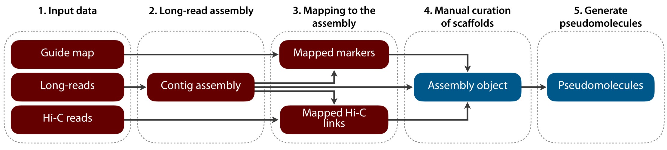
The core algorithm for Hi-C map construction searches for a minimum spanning tree in the graph induced by Hi-C contact matrix and further refines it to include as many scaffolds as possible and to orient them relative to the chromosomal orientation of the guide map. The algorithm has been described in detail by Beier et al. (2017).
In case of questions on the pipeline, contact Martin Mascher.
Short-read TRITEX
The previous version of TRITEX used short-read data.
The old version of this tutorial is available here.
See also the first TRITEX paper.
Installing the required tools
-
The TRITEX pipeline needs to be run on rather powerful Unix servers. It has been tested on servers running recent CentOS Linux version controlled by the SLURM resource scheduler. Some commands like Hi-C read mapping can be submmitted as batch job. Pseudomolecule construction in R requires interactive sessions, either by direct SSH access or use of interactives SLURM sessions. In any case, the use of a terminal multiplexer such as tmux is recommended. Some jobs may run for several days. If Kerberos authentification is used, make sure that tickets are renewed.
-
Install the following software. The pipeline has been run successfully with the versions indicated below. Using the most recent versions should be fine as well.
-
Z shell, 5.0.2
-
GNU Parallel, 20150222, paper
-
gfatools, 0.5
-
Seqtk, 1.0-r76
-
pigz, 2.3.4, parallel gzip
-
BBMap, 37.93
-
faToTwoBit and twoBitInfo, from the UCSC Genome Browser, v.3.69
-
Novosort, 3.06.05. This is commercial software. A single-threaded version is available for free. Novosort is used only in Hi-C read mapping scripts. An alternative using SAMtools instead is available here.
The pipeline assumes that the GNU (as opposed to BSD) versions of common UNIX tools (
coreutils,sed,awk) are used. -
-
The following R packages should be installed and accessible in
.libPaths(). The versions specified are known to work with TRITEX. Newer versions will likely work as well. -
If you want to use the R Shiny app Hi-C map inspector, you need to set up a web server running R Shiny. Refer to the R Shiny manual. Note that setting up a Shiny server is a non-trivial task of Unix systems administration and requires super-user rights.
-
Clone the Bitbucket repository of the TRITEX assembly pipeline. The path to the local copy of the repository will be referenced by
$bitbucketin the code listings. -
The scripts used below have parameters such as
--bedtoolsor--samtools(indicated in the code listings) to specify the absolute paths to the required executables. For better readability, they are omitted from the commands.
Instead of specifying the paths each time you call the scripts, you may also edit the scripts and modify the default paths. We chose not to use executables in $PATH to enforce proper documentation of software versions.
|
Hardware requirements and resource allocation
-
For the hardware requirements of primary contig assembly, we refer to the documentation of hifiasm, a tool commonly used for that purpose. Thirty CPUs and 1 TB RAM will suffice to assemble genomes sequences of 15 GB size within a few days.
-
The Hi-C read mapping script uses
minimap2, which is multi-threaded. More cores translate into shorter run times approximately linearly. Sorting of alignment recordsNovosort(andsamtools) can be speeded up by allocating more RAM for in-memory sorting. Otherwise, temporary disk space is used (which incurs longer run-time because of disk I/O). -
The interactive R sessions for pseudomolecule construction hold large tables of Hi-C links in main memory. For a genome in size range of 5-15 Gb, 500 GB - 1 TB of main memory may be required. Some parts of the pseudomolecule construction are multithreaded (e.g. the
hic_map()function), but savings in run time are negligeable, so running R on an allocation of 1 core will be just fine.
Setting up the folder structure
A folder for each assembly project should be created. We refer to this directory as $projectdir in the code listings below.
The project folder should have the following subdirectory structure. At the start of the pipeline, all folders except "raw_reads" should be empty.
-
raw_reads
-
hifi_reads
-
hic_reads
-
These folders contain the raw reads (or symbolic links to them).
-
-
-
assembly
-
This folder will contain the CCS assembly.
-
-
mapping
-
This folder will contain the results of mapping of Hi-C reads to the HiFi assembly.
-
hic
-
In this folder you should create symbolic links to the Hi-C reads.
-
-
-
-
pseudomolecules
-
This folder will be used to run the pseudomolecule construction section of this tutorial. It will contain the R objects of the assemblies, plots for quality assessment and final pseudomolecule FASTA files.
-
1. Obtaining the input contig assembly
-
Any long-read input assembly will work, but in this tutorial we are going to use HiFi reads with hifiasm.
-
Let’s assemble the HiFi reads with hifiasm. Set up a list of all FASTQ files and run hifiasm. Results will be inside the
$projectdir/assembly/project_name/directory.cd $projectdir/assembly d='$projectdir/raw_reads/hifi_reads' find $d | grep 'fastq.gz$' > hifi_reads.txt reads='hifi_reads.txt' prefix='project_name' threads=30 (1) mkdir $prefix out=$prefix/$prefix xargs -a $reads hifiasm -t $threads -o $out > $out.out 2> $out.err1 Set the number of threads you would like to use. -
Check the stats of contigs and unitigs.
cd $projectdir/assembly/project_name/

grep '^S' project_name.p_ctg.noseq.gfa | cut -f 4 | cut -d : -f 1,3 \
 | tr : '\t' | $bitbucket/shell/n50 > project_name.p_ctg.noseq.gfa.n50 (1)

grep '^S' project_name.p_utg.noseq.gfa | cut -f 4 | cut -d : -f 1,3 \
| tr : '\t' | $bitbucket/shell/n50 > project_name.p_utg.noseq.n50
1 The backslash \ will be used throughout the tutorial to break long shell commands into several lines. When pasting the commands or editing them, make sure that no white space follows the backslash. Otherwise, the shell will interpret the lines as belonging to different commands. Also multi-line commands do not tolerate intervening command line (starting with the hash sign #). -
Convert contig GFA to FASTA and change contig names.
gfa='project_name.p_ctg.gfa'
gfatools gfa2fa $gfa | seqtk rename - contig_ > ${gfa:r}.fa (1)
1 The syntax ${gfa:r}is specific to the Z shell, see the section of the shell manual on expansion and substitution. Very usefyl are:rand:tmodifiers to remove filename extensions and leading pathname components, respectively. The latter works like the UNIX commandbasename.
2. Mapping Hi-C data
-
The first step is to digest in silico the hifiasm assembly with the restriction enzyme used for the preparation of the Hi-C libraries.]
-
If you have Omni-C data, please skip this section and go to the last section, as some commands are adapted.
cd $projectdir/assembly/project_name/
ref='$projectdir/assembly/project_name/project_name.p_ctg.fa' (1)

$bitbucket/shell/digest_emboss.zsh --ref $ref --enzyme 'MboI' --sitelen 4 --minlen 30  (2) (3)
1 $refis the renamed FASTA created in the previous step.2 In the script "digest_emboss.zsh", change the paths to the executables of restrict,bedtoolsandrebase.3 Don’t forget to make sure that the enzyme matches the one used for making your Hi-C libraries. Another common choice is --enzyme 'DpnII' --sitelen 4. -
Put the gzipped FASTQ files of the Hi-C reads (or symbolic links to them) of the Hi-C reads in the folder "hic".
-
Now start the Hi-C mapping.
cd $projectdir/mapping/
ref='$projectdir/assembly/project_name/project_name.p_ctg.fa'
map='$bitbucket/shell/run_hic_mapping.zsh' (1)
bed=${ref:r}_MboI_fragments_30bp.bed (2)
cd $projectdir

$map --threads 64 --mem '200G' --linker "GATCGATC" --ref $ref --bed $bed --tmp $TMPDIR hic (3) (4)| 1 | You need to specify in the script the paths to the following executables: Cutadapt (--cutadapt), bgzip (--bgzip), Minimap2 (--minimap), Novosort (--novosort), SAMtools (--samtools), and BEDTools (--bedtools). |
| 2 | Use the BED file with the in silico digest for the correct restriction enzyme. Using the wrong enzyme will give wrong results. |
| 3 | Specify correct linker sequences that is created by ligation of fill-in overhangs during the Hi-C protocol. If HindIII was used, the correct linker is AAGCTAGCTT; if DpnII was used, the linker is GATCGATC. |
| 4 | The temporary directory needs to be large enough to hold huge BAM files (dozens of GB). |
3. Creating the guide map table
The guide map table can be from a genetic map or from a reference genome. The expected format in R is as follows:
| css_contig | popseq_cM | sorted_genome | css_contig_length | popseq_alphachr | sorted_arm | popseq_chr | sorted_alphachr | sorted_chr | sorted_lib |
|---|---|---|---|---|---|---|---|---|---|
<char> |
<num> |
<char> |
<int> |
<char> |
<lgcl> |
<int> |
<char> |
<int> |
<char> |
seq_1 |
0.0000595 |
D |
119 |
7D |
NA |
21 |
7D |
21 |
7D |
3.1. If you have a genetic map
-
Follow these steps if you already have a guide map. We are going to adjust it to the above format to be used in TRITEX.
-
If you plan on using a reference genome to build a guide map, go to the next section.
-
An example file is available here (MaizeB73_guidemap_marker_IBM.Rds).
-
You will need a BED file with the genomic positions of your markers. The fourth column should contain IDs like "seq_N", where N goes from 1 to the number of markers.
-
Most steps will be done in R from now on. If you are unsure whether a command should be pasted to the R or the shell prompt, hover with the mouse over the code listings. SH or R should appear in the top-right corner.
# read the BED file containing the marker regions
fread('genetic_map.bed') -> p

setnames(p, c("agp_chr", "agp_start", "agp_end", "seq"))
p[, .(css_contig=seq, popseq_cM=(agp_start+agp_end)/2/1e6, #set pseudo-cM as Mb position
    sorted_genome = as.character(NA),
    css_contig_length = agp_end - agp_start,
    popseq_alphachr = as.character(agp_chr), # it needs to be character column
    sorted_arm = NA) ] -> pp

pp[,popseq_chr:=as.integer(popseq_alphachr)]
pp[, sorted_alphachr := popseq_alphachr]
pp[, sorted_chr := popseq_chr]
pp[, sorted_lib := popseq_alphachr]

# Adjust any other columns based on your species.

# Save as RDS file for use in TRITEX pipeline
saveRDS(pp, "project_name_pseudopopseq.Rds")
Now you should map the guide map sequences to the contig assembly. Skip to this section.
3.2. If you are using a reference genome as guide map
-
In case you want to create a guide map from an available reference genome, first you need to obtain single-copy 100bp regions.
-
If you already have a genetic map, you can skip this step and go to the next section.
mask='$bitbucket/miscellaneous/mask_assembly.zsh' (1)
fa='$projectdir/reference_assembly.fasta' (2)
bed="${fa:t:r}_masked_noGaps.bed"
out="${fa:t:r}_singlecopy_100bp"

$mask --mem 300G --fasta $fa --mincount 2 --out "."

awk '$3 - $2 >= 100' $bed | grep -v chrUn | awk '{print $0"\tseq_"NR}' \
| tee $out.bed | bedtools getfasta -fi $fa -bed /dev/stdin -name -fo $out.fasta| 1 | You need to specify the paths to the following executables: BBDuk (bbduk), fatotwobit (bit), twobitinfo (tbinfo), kmercountexact.sh (from BBMap) (kmer), SAMtools (samtools), and BEDTools (bedtools). |
| 2 | Use a reference assembly for the studied species. |
-
Most steps will be done in R from now on. If you are unsure whether a command should be pasted to the R or the shell prompt, hover with the mouse over the code listings. SH or R should appear in the top-right corner.
-
Now it is time to build the pseudo POPSEQ file (the guide map), which is used as input for the TRITEX pipeline.
-
Here is an example file of how your guide map should look like.
# Read single-copy regions generated in last step
f<-'reference_assembly_singlecopy_100bp.bed'
fread(f) -> p
setnames(p, c("agp_chr", "agp_start", "agp_end", "seq"))

# Change chromosome names to their respective chr numbers
# These are example names from maize

ids <- c("NC_050096.1",
         "NC_050097.1",
         "NC_050098.1",
         "NC_050099.1",
         "NC_050100.1",
         "NC_050101.1",
         "NC_050102.1",
         "NC_050103.1",
         "NC_050104.1",
         "NC_050105.1")

for (i in 1:10){
  p[grepl(ids[i], agp_chr), agp_chr:=as.integer(i)]
}

# This is for unplaced scaffolds, assigning them as "NA"
p[grepl("NW", agp_chr), agp_chr:=as.integer(NA)]

p[, .(css_contig=seq, popseq_cM=(agp_start+agp_end)/2/1e6, #set pseudo-cM as Mb position
    sorted_genome = as.character(NA),
    css_contig_length = agp_end - agp_start,
    popseq_alphachr = as.character(agp_chr), # it needs to be character column
    sorted_arm = NA) ] -> pp

pp[,popseq_chr:=as.integer(popseq_alphachr)]
pp[, sorted_alphachr := popseq_alphachr]
pp[, sorted_chr := popseq_chr]
pp[, sorted_lib := popseq_alphachr]

# Save as RDS file for use in TRITEX pipeline
saveRDS(pp, "project_name_pseudopopseq.Rds")
3.3. Mapping the guide map sequences to the genome
-
Independently of how you obtained your guide map, you should map the marker sequences to the contig assembly.
-
The output PAF file will be input into R into the next step.
ref='$projectdir/assembly/project_name/project_name.p_ctg.fa'
qry='reference_assembly_singlecopy_100bp.fasta' # this is the guide map sequence file
size='20G'
mem='5G'
threads=30
prefix=${ref:t:r}_project_name

{
minimap -t $threads -2 -I $size -K$mem -x asm5 $ref $qry | bgzip > $prefix.paf.gz
} 2> $prefix.err &
4. Creating the assembly object
-
Now we are going to load the contig assembly, guide map and the Hi-C alignment records into R to create the assembly object.
-
All subsequent steps should be carried out in the working directory
$projectdir/pseudomolecules/. -
First load all the necessary datasets into R.
# Load the R functions for pseudomolecule construction.
source("$bitbucket/R/pseudomolecule_construction.R") (1)

# Import the guide map.
readRDS('$projectdir/project_name_pseudopopseq.Rds') -> popseq

# Read contig lengths
f <- '$projectdir/assembly/project_name/project_name.p_ctg.fa.fai'
fread(f, head=F, select=1:2, col.names=c("scaffold", "length")) -> fai

# Read guide map alignment.
f <- '$projectdir/assembly/project_name/project_name_ctg.paf.gz' (2)
read_morexaln_minimap(paf=f, popseq=popseq, minqual=30, minlen=500, prefix=F) -> morexaln (3)

# Read Hi-C links
dir <- '$projectdir/hic'
fread(paste('find', dir, '| grep "_pairs.tsv.gz$" | xargs zcat'),
       header=F, col.names=c("scaffold1", "pos1", "scaffold2", "pos2")) -> fpairs
1 Note that $bitbucket,$projectdirand$assemblywill not be evaluated as variables by R here and in all other instances below. Replace them always with a correct path by modifying the command with a text editor before running it.2 Note that IDs in this file should be the same as in the guide map. Modify them if needed. 3 Change the minlenparameter depending on the length of the guide map marker size. -
Now initialize and save the assembly.
# Init and save assembly, replace species with the right one. Here we are going to use "maize".
init_assembly(fai=fai, cssaln=morexaln, fpairs=fpairs) -> assembly
anchor_scaffolds(assembly = assembly, popseq=popseq, species="maize") -> assembly (1)
add_hic_cov(assembly, binsize=1e4, binsize2=1e6, minNbin=50, innerDist=3e5, cores=1) -> assembly  (2) (3)
saveRDS(assembly, file="assembly.Rds") (4)
| 1 | Possible values for the species parameter are: 'barley', 'wheat' (works for A genome species, T. turgidum and T. aestivum), 'maize', 'rye', 'oats_new' (chromosomes 1 to 7, subgenomes A, B and D), 'avena_barbata', 'hordeum_bulbosum', 'faba_bean', 'lolium', and 'rapeseed'. More species can be accomodated by re-defining the function chrNames(). Type chrNames to see its source code. The only use of species is to map numeric chromosome IDs to proper names, e.g. 1 to 1H in barley (see the note by
Linde-Laursen to see why this makes a difference) or 21 to 7D. |
| 2 | Change number of cores according to match your allocated resources. Don’t forget to change it in the next steps also. |
| 3 | binsize is the resolution at which physical coverage is calculated. binsize2 is the size of batches for parallelization; smaller values decrease memory consumption. |
| 4 | It is recommended to prefix the names of the RDS files created in this and later steps with the current date (e.g. "220801_assembly.Rds") to distinguish different versions. |
4.1. Breaking chimeric scaffolds
-
Generate diagnostic plots to check for chimeras in the input assembly. If sequences from different chromosomes are joined, the chimeric scaffolds will have guide map markers from more than one chromosome.
# Create diagnostic plots for contigs longer than 1 Mb.
assembly$info[length >= 1e6, .(scaffold, length)][order(-length)] -> s
plot_chimeras(assembly=assembly, scaffolds=s, species="maize",
	refname="B73", autobreaks=F, mbscale=1, file="assembly_1Mb.pdf", cores=1) (1)

# Diagnostic plots for putative chimeras with strong drops in Hi-C coverage.
assembly$info[length >= 1e6 & mri <= -3, .(scaffold, length)][order(-length)] -> s
plot_chimeras(assembly=assembly, scaffolds=s, species="maize",
	refname="B73", autobreaks=F, mbscale=1, file="assembly_chimeras.pdf", cores=1)
1 Don’t forget to change species and reference name. -
Check the plots and search for drops in Hi-C coverage, misalignments and chimeras. For each case, assign the PDF page number from "assembly_1Mb.pdf" and the positions where it needs breaking.
-
For instance, in this example, the scaffolds that need to be broken are on pages 3, 6, and 9. We need to change the bins where the scaffold should be splitted.
assembly$info[length >= 1e6, .(scaffold, length)][order(-length)] -> ss i=3 # page number in PDF ss[i]$scaffold -> s # change the bin position observed in the plots assembly$cov[s, on='scaffold'][bin >= 10e6 & bin <= 22e6][order(r)][1, .(scaffold, bin)] -> b i=6 # page number in PDF ss[i]$scaffold -> s rbind(b, assembly$cov[s, on='scaffold'][bin >= 40e6 & bin <= 45e6][order(r)][1, .(scaffold, bin)])->b i=9 # page number in PDF ss[i]$scaffold -> s rbind(b, assembly$cov[s, on='scaffold'][bin >= 1e6 & bin <= 9e6][order(r)][1, .(scaffold, bin)])->b # Rename column and plot again to double-check the breakpoints are correct setnames(b, "bin", "br") plot_chimeras(assembly=assembly, scaffolds=b, br=b, species="maize", refname="B73", mbscale=1, file="assembly_chimeras_final.pdf", cores=1) -
After checking if the break points are in the right places, proceed with breaking the scaffolds.
break_scaffolds(b, assembly, prefix="contig_corrected_v1_", slop=1e4, cores=1, species="maize") -> assembly_v2
saveRDS(assembly_v2, file="assembly_v2.Rds") (1)
1 This will create a new file for the assembly. -
Now we make the Hi-C contact matrix, or Hi-C map. Three files will be generated: a PDF with the intrachromosomal plots, a PDF with the interchromosomal plots, and a file to be loaded into R Shiny Map inspector (
*_export.Rds).fbed <- '$projectdir/assembly/project_name/project_name.p_ctg_MboI_fragments_30bp.bed' read_fragdata(info=assembly_v2$info, file=fbed) -> frag_data # Consider only contigs >= 1 Mb first frag_data$info[!is.na(hic_chr) & length >= 1e6, .(scaffold, nfrag, length, chr=hic_chr, cM=popseq_cM)] -> hic_info hic_map(info=hic_info, assembly=assembly_v2, frags=frag_data$bed, species="maize", ncores=1, min_nfrag_scaffold=30, max_cM_dist = 1000, binsize=2e5, min_nfrag_bin=10, gap_size=100) -> hic_map_v1 saveRDS(hic_map_v1, file="hic_map_v1.Rds") # Make the Hi-C plots, files will be placed in your working directory. snuc <- '$projectdir/assembly/project_name/project_name.p_ctg_MboI_fragments_30bp_split.nuc.txt' hic_plots(rds="hic_map_v1.Rds", assembly=assembly_v2, cores=1, species="maize", nuc=snuc) -> hic_map_v2 -
Let’s do a second round of checking for chimeras. Broken scaffolds in the last step are renamed in the plots. It might not be necessary to break any more scaffolds; in this case, just check the plots and if everything is alright, proceed to decrease the contig size to 500 kb.
# If you'd like to plot specific contigs: data.table(scaffold=c('contig_corrected_v1_53', 'contig_corrected_v1_24', 'contig_corrected_v1_5', 'contig_corrected_v1_76') -> ss # If you'd like to check them all again: assembly_v2$info[length >= 1e6, .(scaffold, length)][order(-length)] -> ss plot_chimeras(assembly=assembly_v2, scaffolds=ss, species="maize", refname="B73", autobreaks=F, mbscale=1, file="assembly_v2_chimeras.pdf", cores=1) # In case there are more chimeras, proceed like the previous step. Assign `i` with the PDF page and don't forget to change the bin. Otherwise, plot the Hi-C map with contigs >= 500 kb. -
If another round of breaking scaffolds is needed, you can just run the previous block again. Don’t forget to change the output files and object names (assembly_vX, hic_map_vX).
-
If no more chimeras are found, proceed to decreasing the size to 500 kb.
frag_data$info[!is.na(hic_chr) & length >= 5e5, .(scaffold, nfrag, length, chr=hic_chr, cM=popseq_cM)] -> hic_info

hic_map(info=hic_info, assembly=assembly_v2, frags=frag_data$bed, species="maize",
	ncores=1, min_nfrag_scaffold=30, max_cM_dist = 1000, binsize=2e5,
	min_nfrag_bin=10, gap_size=100) -> hic_map_v2 (1)

saveRDS(hic_map_v2, file="hic_map_v2.Rds") (1)

snuc <- '$projectdir/assembly/project_name.p_ctg_MboI_fragments_30bp_split.nuc.txt'
hic_plots("hic_map_v2.Rds", assembly=assembly_v2, cores=1,
	species="maize", nuc=snuc) -> hic_map_v2 (1)


# Exporting to Excel the table that will be used for manual curation.
write_hic_map(rds="hic_map_v2.Rds", file="hic_map_v2.xlsx", species="maize")
1 Don’t forget to put the correct object name here.
5. Manual curation of scaffolds
Now that we have the scaffolded assembly, we are going to check if there are any inversions, extra contigs, or misplaced contigs. To do so, we can check the Hi-C plots generated in the last step coupled with a collinearity plot of scaffolds (the AGP, hic_map object) to the guide map. It is also possible to use the R Shiny Map Inspector app to zoom in the Hi-C intrachromosomal plots to check the contigs that need to be changed.
5.1. Collinearity plots
-
This step is optional, yet recommended. It will help spot inverted or misplaced contigs. The collinearity plots will show marker positions against the assembly. It is possible to check the alignments and spot inverted/misplaced contigs. You can do this anytime you want to check the collinearity to the assembly. Remember that your assembly might be different compared to the reference you used, so always check the Hi-C contact maps also.
assembly_v2$cssaln[, .(scaffold, pos, guide_chr=paste0("chr", "", popseq_alphachr), guide_pos=popseq_cM)] -> x  (1)
hic_map_v2$agp[, .(scaffold, agp_start, agp_end, orientation, agp_chr)][x, on="scaffold"]-> x (2)

x[orientation == 1, agp_pos :=  agp_start + pos]
x[orientation == -1, agp_pos :=  agp_end - pos]
x[agp_chr == guide_chr] -> x

pdf("hic_map_v2_3_vs_assembly_v2.pdf", height=3*3, width=3*3)
par(mar=c(5,5,3,3))
lapply(chrNames(species="maize", agp=T)$agp_chr[1:10], function(i){   (3)
print(i)
x[i, plot(pch=".", main=i, agp_pos/1e6, guide_pos/1e6, xlab="Hi-C AGP", ylab="guide", las=1, bty='l'), on="agp_chr"]
hic_map_v2$agp[agp_chr == i & gap == T][, abline(v=agp_start/1e6, col="gray")] (2)
})
dev.off()
1 Change assembly name accordingly. 2 Change Hi-C map name accordingly. 3 Change species and number of chromosomes [1:10] accordingly.
5.2. Checking Hi-C maps
-
You can use Map Inspector Shiny app or the intrachromosomal plots for manual curation. Genomic regions containing putatively chimeric scaffolds can be clicked on to get their names and pinpoint the sites of culpable misjoins.
-
The source code required for deploying Hi-C Map Inspector on an R Shiny server is contained in
$bitbucket/R/map_inspector.Rmd. You need to modify the paths to the data directory and the default map object. -
You’ll want to check for inversions near scaffold borders (grey lines).
-
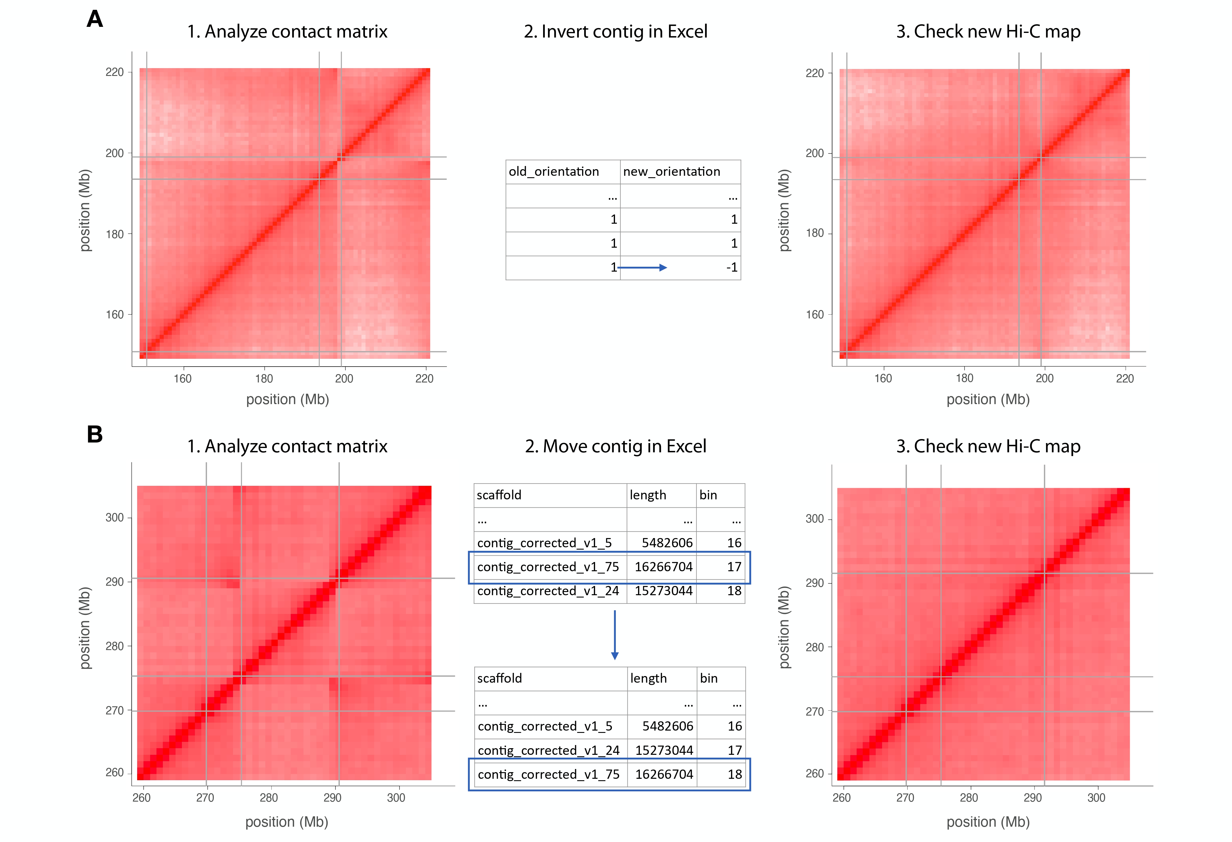
When modifications are spotted, change the Excel file generated in the last steps.
-
If an inverted contig is spotted, the column "new_orientation" on the table must be changed (Fig. 2A).
-
If there is a misplaced contig, the row containing it should be moved (don’t forget to change the bin number order) (Fig. 2B).
-
If there is an extra contig, you can remove it from the chromosome sheet and put it in the "chrUn" sheet. This will move this contig to the unanchored contig portion of the genome.
-
After making the changes, import the Excel file again and proceed with mapping.
read_hic_map(rds="hic_map_v2.Rds", file="hic_map_v2_edit.xlsx") -> nmap diff_hic_map(rds="hic_map_v2.Rds", nmap, species="maize") hic_map(species="maize", agp_only=T, map=nmap) -> hic_map_v3 saveRDS(hic_map_v3, file="hic_map_v3.Rds") # Final Hi-C plots. You can check if the inverted scaffolds are correct. snuc <- '$projectdir/assembly/project_name.p_ctg_MboI_fragments_30bp_split.nuc.txt' hic_plots(rds="hic_map_v3.Rds", assembly=assembly_v2, cores=1, species="maize", nuc=snuc) -> hic_map_v3 -
If there are still wrong contigs, you can make new modifications to the Excel file and repeat this block until there are no more changes needed. You can make another collinearity plot to help you.
6. Compiling pseudomolecules
-
First let’s get some stats of the pseudomolecules.
hic_map_v3$agp[agp_chr != "chrUn" & gap == F][, .("Ncontig" = .N, "N50 (Mb)"=round(n50(scaffold_length/1e6), 1), "max_length (Mb)"=round(max(scaffold_length/1e6),1), "min_length (kb)"=round(min(scaffold_length/1e3),1)), key=agp_chr] -> res hic_map_v3$chrlen[, .(agp_chr, "length (Mb)"=round(length/1e6, 1))][res, on="agp_chr"] -> res setnames(res, "agp_chr", "chr") hic_map_v3$agp[gap == F & agp_chr != "chrUn"][, .("Ncontig" = .N, "N50 (Mb)"=round(n50(scaffold_length/1e6), 1), "max_length (Mb)"=round(max(scaffold_length/1e6),1), "min_length (kb)"=round(min(scaffold_length/1e3),1))][, agp_chr := "1-10"] -> res2 hic_map_v3$chrlen[, .(agp_chr="1-10", "length (Mb)"=round(sum(length)/1e6, 1))][res2, on="agp_chr"] -> res2 setnames(res2, "agp_chr", "chr") hic_map_v3$agp[gap == F & agp_chr == "chrUn"][, .(chr="un", "Ncontig" = .N, "N50 (Mb)"=round(n50(scaffold_length/1e6), 1), "max_length (Mb)"=round(max(scaffold_length/1e6),1), "min_length (kb)"=round(min(scaffold_length/1e3),1), "length (Mb)"=sum(scaffold_length/1e6))] -> res3 rbind(res, res2, res3) -> res write.xlsx(res, file="hic_map_v3_pseudomolecule_stats.xlsx") -
And finally compile the pseudomolecules. The FASTA file will be placed inside the directory assigned in "output".
fasta <- '$projectdir/assembly/project_name/project_name.p_ctg.fa' # this is the contig assembly
sink("pseudomolecules_v1.log") (1)
compile_psmol(fasta=fasta, output="pseudomolecules_v1",
	hic_map=hic_map_v3, assembly=assembly_v2, cores=1)
sink() (1)
| 1 | That opens and closes a log file. |
Your genome assembly is ready!
7. Mapping Omni-C data
This section is about using Omni-C data instead of Hi-C.
ref='$projectdir/assembly/project_name/project_name.p_ctg.fa'
mem='300G'
out='OmniC'

cd $projectdir/mapping/

./run_hic_mapping_omni.zsh --threads 20 --mem '100G' --ref $ref --tmp $TMPDIR hic


bam='$projectdir/mapping/hic_reads.bam'

samtools view -q 10 -F 3332 $bam | cut -f -4 \
| awk NF | awk 'old != $1 {old=$1; printf "\n"$0; next} {printf "\t"$0}' \
| awk -F '\t' 'NF == 8' | cut -f 3,4,7,8 | awk '{printf "%s\t%20d\t%s\t%20d\n", $1,1+($2 / 10000)*10000,$3,($4 / 10000)*10000}' \
| gzip > ${bam:r}_pairs.txt.gz


# make BED file of 10kb bins
bedtools makewindows -w 10000 -g $projectdir/assembly/project_name/project_name.p_ctg.fasta.fai > project_name.p_ctg_rename_assembly_10kb.bed (1)

# get BEDTools nuc output for 10 kb bins
ref='$projectdir/assembly/project_name/project_name.p_ctg.fa'
bed='project_name.p_ctg_rename_assembly_10kb.bed'
awk 'BEGIN{OFS="\t"} {print $0, $1":"$2"-"$3}' $bed \
| bedtools nuc -bed - -fi $ref > ${bed:r}_split.nuc.txt (2)| 1 | This will be imported into R as "fbed". |
| 2 | This will be imported into R as "snuc". |
If you need to downsample the Omni-C data, do this after importing Omni-C data into R.
# down sample
fpairs[seq(1, .N, 10)] -> fpairs2
copy(fpairs2) -> x
setnames(x, sub("1", "3", names(x)))
setnames(x, sub("2", "1", names(x)))
setnames(x, sub("3", "2", names(x)))
rbind(fpairs2, x) -> fpairs2